Fit Attenuation Curves

The dust_attenuation package is built on the astropy.modeling package. Fitting is done in the standard way for this package where the model is initialized with a starting point (either the default or user input), the fitter is chosen, and the fit performed.

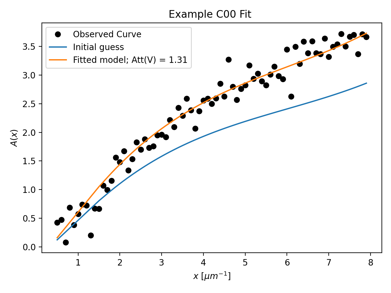
Example: C00 Fit

In this example, a mock attenuation curve (C00 model with noise) is fitted with the C00 model.

import matplotlib.pyplot as plt
import numpy as np

from astropy.modeling.fitting import LevMarLSQFitter
import astropy.units as u

from dust_attenuation.averages import C00

# Create mock attenuation curve with C00 and Av = 1.3 mag
# Better sampling using wavenumbers
x = np.arange(0.5, 8.0, 0.1)/u.micron
# Convert to microns
x = 1/x

att_model = C00(Av=1.3)
y = att_model(x)
# add some noise
noise = np.random.normal(0, 0.2, y.shape)
y += noise

# initialize the model
c00_init = C00()

# pick the fitter
fit = LevMarLSQFitter()

# fit the data to the FM90 model using the fitter
#   use the initialized model as the starting point
c00_fit = fit(c00_init, x.value, y)

print ('Fit results:\n', c00_fit)
# plot the observed data, initial guess, and final fit
fig, ax = plt.subplots()

ax.plot(1/x, y, 'ko', label='Observed Curve')
ax.plot(1/x.value, c00_init(x.value), label='Initial guess')
ax.plot(1/x.value, c00_fit(x.value),
        label='Fitted model; Att(V) = %.2f' % (c00_fit.Av.value))

ax.set_xlabel('$x$ [$\mu m^{-1}$]')
ax.set_ylabel('$A(x)$')

ax.set_title('Example C00 Fit ')

ax.legend(loc='best')
plt.tight_layout()
plt.show()

(Source code, png, hires.png, pdf)

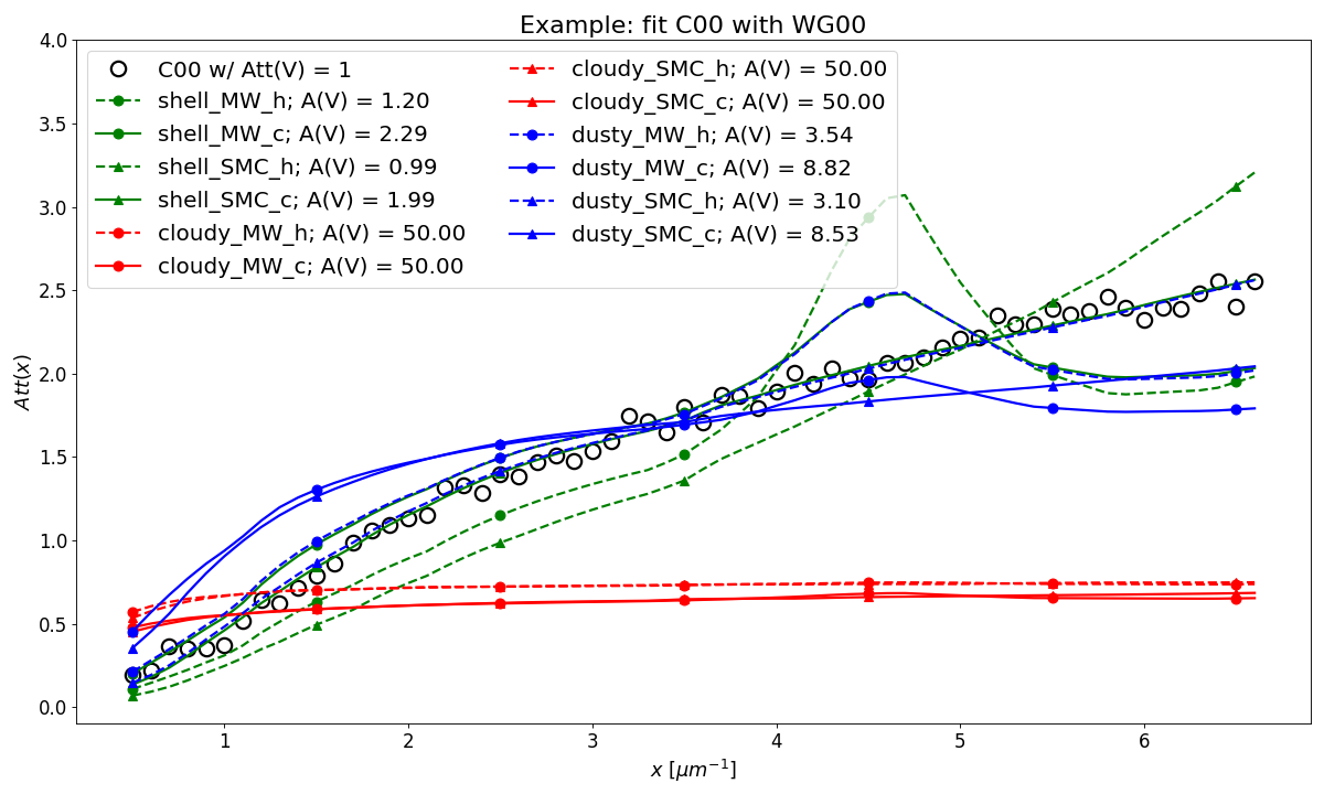
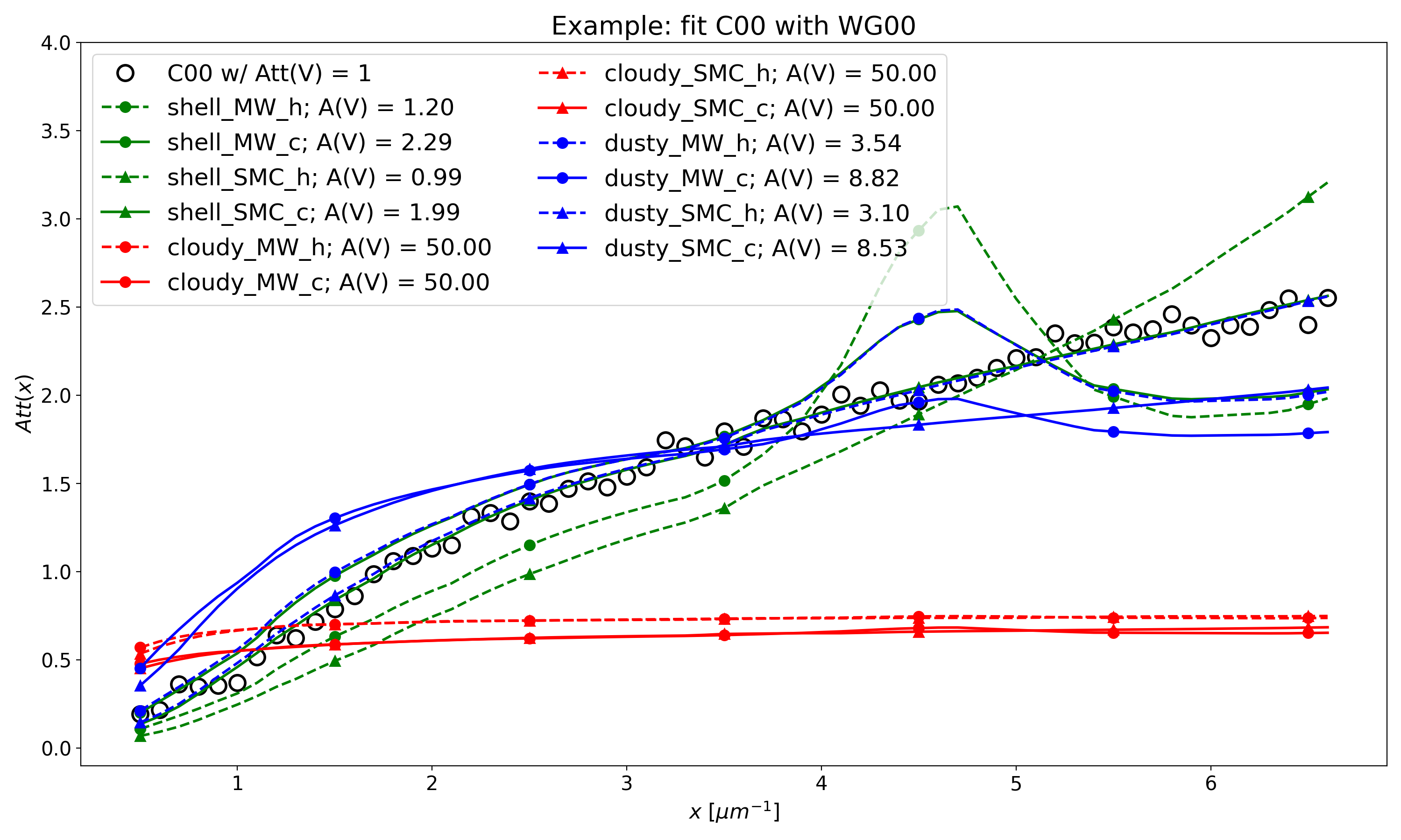
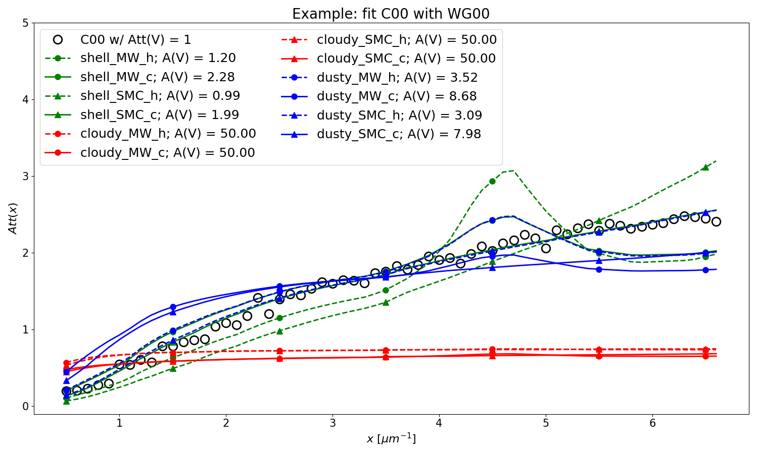
Example: Use WG00 to fit C00

In this example, we are using the WG00 attenuation curves to fit the Calzetti attenuation curve (C00 model) with Att(V) = 1 mag and noise. The two WG00 configurations that best fit both have SMC-type dust and are the SHELL geometry with clumpy dust distribution and the DUSTY geometry with homogeneous dust distribution. The best fit values of the amount of dust in the system are given as the model radial A(V) values.

import numpy as np
import matplotlib.pyplot as plt
from astropy.modeling.fitting import LevMarLSQFitter
import astropy.units as u

from dust_attenuation.averages import C00
from dust_attenuation.radiative_transfer import WG00

# Generate the C00 curve with Av = 1 mag and add some noise
x = np.arange(1/2, 1/0.15, 0.1)/u.micron
x= 1/x
att_model = C00(Av = 1)
y = att_model(x)
noise = np.random.normal(0, 0.05, y.shape)
y += noise

# Wavelength of V band
x_Vband = 0.55

geometries = ['shell', 'cloudy', 'dusty']
dust_types = ['MW', 'SMC']
dust_distribs = ['homogeneous', 'clumpy']

# pick the fitter
fit = LevMarLSQFitter()

# plot the observed data, initial guess, and final fit
plt.figure(figsize=(15, 9))

plt.plot(1/x, y, 'ko', label='C00 w/ Att(V) = 1', markersize=12,
         fillstyle='none', markeredgewidth=2)

# Loop over the different configurations
for geo in geometries:
    for dust in dust_types:
        for distrib in dust_distribs:

            label = geo + '_' + dust + '_' + distrib[0]

            if geo == 'cloudy': color = 'red'
            elif geo == 'dusty': color = 'blue'
            elif geo == 'shell': color = 'green'

            if dust == 'MW': marker = 'o'
            elif dust == 'SMC': marker = '^'

            if distrib == 'homogeneous': ls = '--'
            if distrib == 'clumpy':  ls = '-'

            WG00_init = WG00(tau_V = 2.0, geometry = geo,
                             dust_type = dust,
                             dust_distribution = distrib)

            # fit the data to the WG00 model using the fitter
            #   use the initialized model as the starting point
            WG00_fit = fit(WG00_init, x.value, y)

            # add best fitting Att(V) value to label
            #   since the C00 model is in Att units, then best fit
            #   tau_V value will actually be Att(V)
            label = '%s; A(V) = %.2f' % (label, WG00_fit.tau_V.value)

            plt.plot(1/x.value, WG00_fit(x.value),
                     label = label, ls = ls, lw = 2, color = color,
                     marker = marker, markevery = 10, markersize = 8 )


plt.xlabel('$x$ [$\mu m^{-1}$]', size=16)
plt.ylabel(r'$Att(x)$', size=16)

plt.ylim(-0.1, 4.0)

plt.title('Example: fit C00 with WG00', size=20)
plt.tick_params(labelsize=15)
plt.legend(loc='upper left', fontsize=18, ncol=2)
plt.tight_layout()
#plt.show()

(Source code, png, hires.png, pdf)

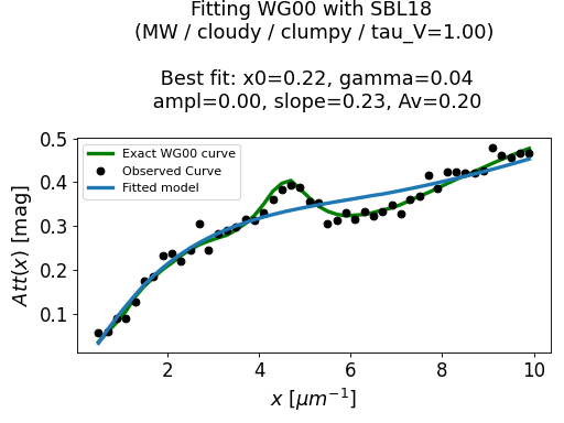
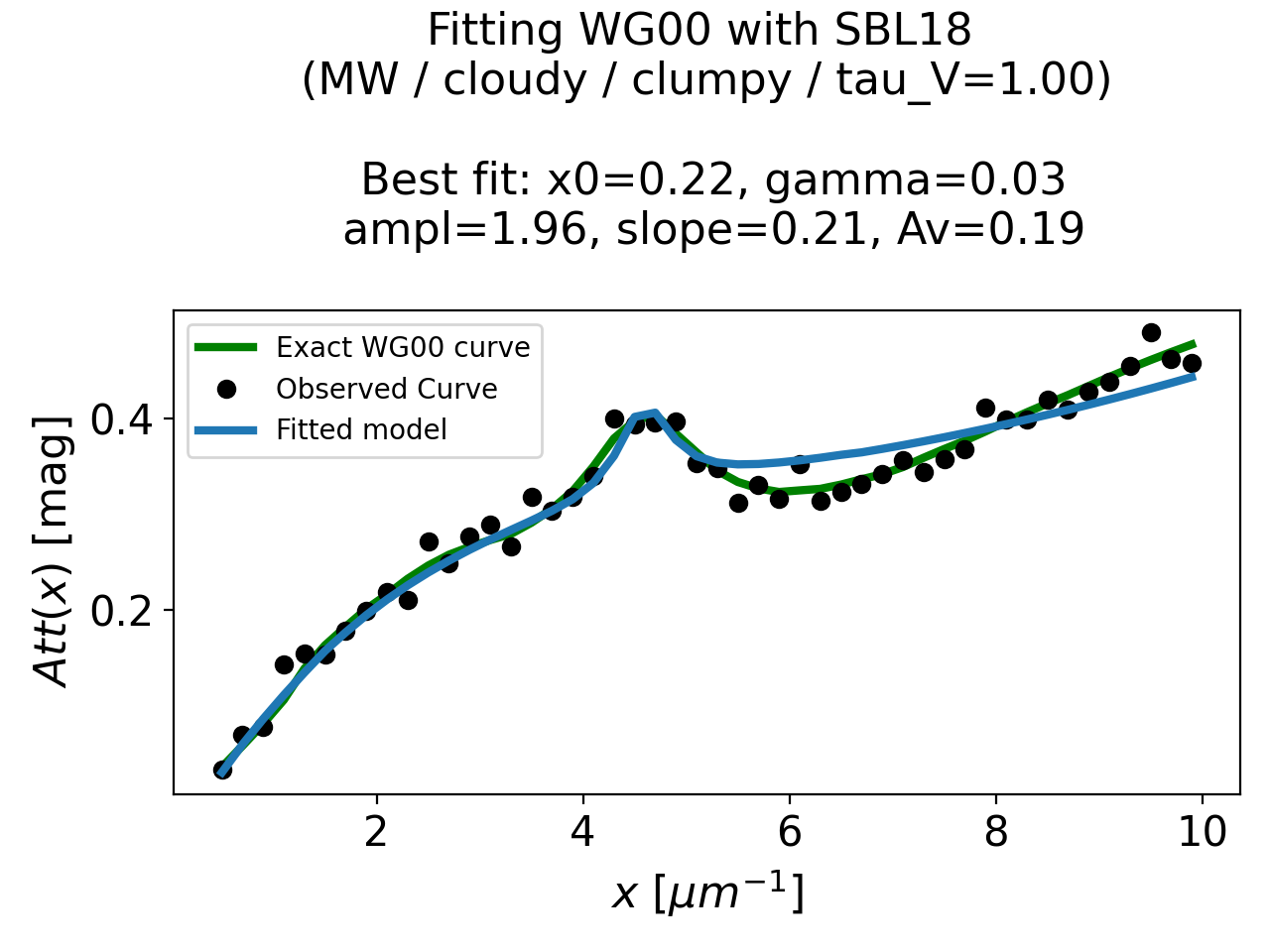
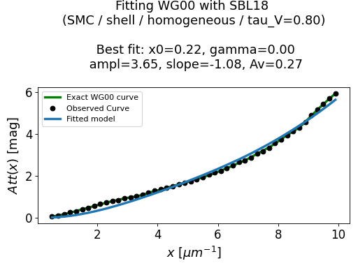
Example: Use SBL18 to fit WG00

In this example, we are using the modified Calzetti law from N09, with the modification of SBL18 to fit some attenuation curves computed with the radiative transfer model of WG00. We chose 2 attenuation curves from the WG00 models:

• MW dust type with the CLOUDY geometry, a clumpy local dust distribution and tau_V=1

• SMC dust type with the SHELL geometry, an homogeneous local dust distribution and tau_V=0.8

The best fit values are given in the title of each figure:

• gamma: width (FWHM) of the UV bump (in microns)

• ampl: amplitude of the UV bump

• slope: slope of the power law

• Av: amount of dust in V band (in mag)

import numpy as np
import matplotlib.pyplot as plt
from astropy.modeling.fitting import LevMarLSQFitter
import astropy.units as u

from dust_attenuation.shapes import SBL18
from dust_attenuation.radiative_transfer import WG00

# Generate an attenuation curve with WG00 and add some noise
x = np.arange(1/2, 1/0.1, 0.2) / u.micron

x = 1 / x

# Wavelength of V band
x_Vband = 0.55

geometry = ['cloudy', 'shell']
dust_type = ['MW', 'SMC']
dust_distrib = ['clumpy', 'homogeneous']
tau_V = [1, 0.8]


for dust, geo, distrib, tau in zip(dust_type, geometry,
                                   dust_distrib, tau_V):

    # Create WG00 attenuation curves
    # initialize the model
    att_model = WG00(tau_V = tau, geometry = geo,
                     dust_type = dust,
                     dust_distribution = distrib)

    y_nonoise = att_model(x)
    noise = np.random.normal(0, 0.015, y_nonoise.shape)
    y = y_nonoise + noise

    # initialize the fitting model
    att_init = SBL18(Av=1, slope=-0.5,ampl=3)

    # Fix central wavelength of the UV bump
    att_init.x0.fixed = True

    # pick the fitter
    fit = LevMarLSQFitter()

    # fit the data to the FM90 model using the fitter
    # use the initialized model as the starting point
    att_fit = fit(att_init, x.value, y, maxiter=10000, acc=1e-20)

    # plot the observed data, initial guess, and final fit
    #fig, ax = plt.subplots(figsize=(10,6))
    fig, ax = plt.subplots()

    ax.plot(1/x, y_nonoise, color='green', label='Exact WG00 curve', lw=3)
    ax.plot(1/x, y, 'ko', label='Observed Curve', lw=0.3)
    ax.plot(1/x.value, att_fit(x.value), label='Fitted model', lw=3)

    ax.set_xlabel('$x$ [$\mu m^{-1}$]', size=16)
    ax.set_ylabel('$Att(x)$ [mag]', size=16)
    ax.tick_params(labelsize=15)
    ax.set_title('Fitting WG00 with SBL18 \n(%s / %s / %s / tau_V=%.2f)\n\n Best fit: x0=%.2f, gamma=%.2f\n ampl=%.2f, slope=%.2f, Av=%.2f\n ' % (dust, geo, distrib, tau, att_fit.x0.value, att_fit.gamma.value, att_fit.ampl.value, att_fit.slope.value, att_fit.Av.value), size=16)

    ax.legend(loc='best')
    plt.tight_layout()
    plt.show()

(Source code)

(png, hires.png, pdf)

(png, hires.png, pdf)

More Examples

TBA.